
Features
Everything between the microscope and the figure
SPATIALTM 2 covers the whole path, from upload to registration, segmentation, phenotyping, spatial analysis and export, so nothing gets lost in handovers between tools.

Your workflow
The analysis runs in nine stages, each with several methods. Select your experiment to see which methods it uses.
Inputs
Assay and modality
- consecutive sections
Registration
Align what belongs together
QC
Before you commit to a run
Segment and annotate
Cells, pathology, regions
- from images
- from transcripts
- regions
- structures
- trained on your tissue
Extract features
Per cell
- by radius
Represent and harmonise
Before phenotyping
- UMAP
- t-SNE
- PCA
- scVI
Phenotype and cluster
Name the populations
- Leiden
- PhenoGraph
Spatial discovery
Where they sit
- UTAG
- BANKSY
Compare cohorts
Across groups and conditions
- regenerates with the data
Segmentation
Cells with morphology, not just nuclei
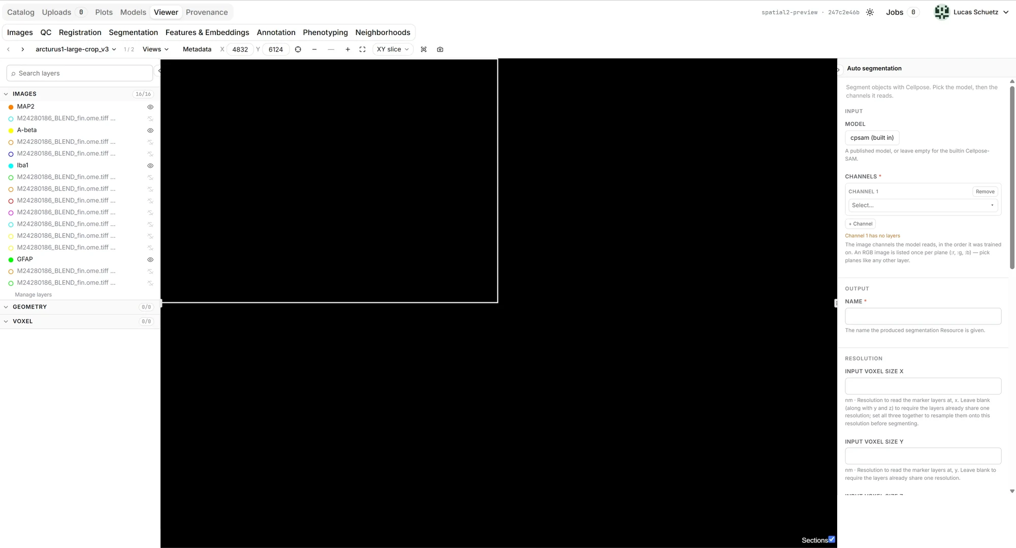
Segment from any channel on which cell outlines can be made out: antibody-derived stains such as CD45, NeuN, IBA1, GFAP and DAPI, or H&E and haematoxylin. Combine several markers for one segmentation and add a nucleus channel if you like. The result keeps branching and process morphology, so morphometric features of neurons and glia stay measurable.
- Multi-marker segmentation
- Nuclear and membrane channels
- Neuron and glia morphology
- Whole slide, no tiling artefacts
Registration
Elastic alignment at any size
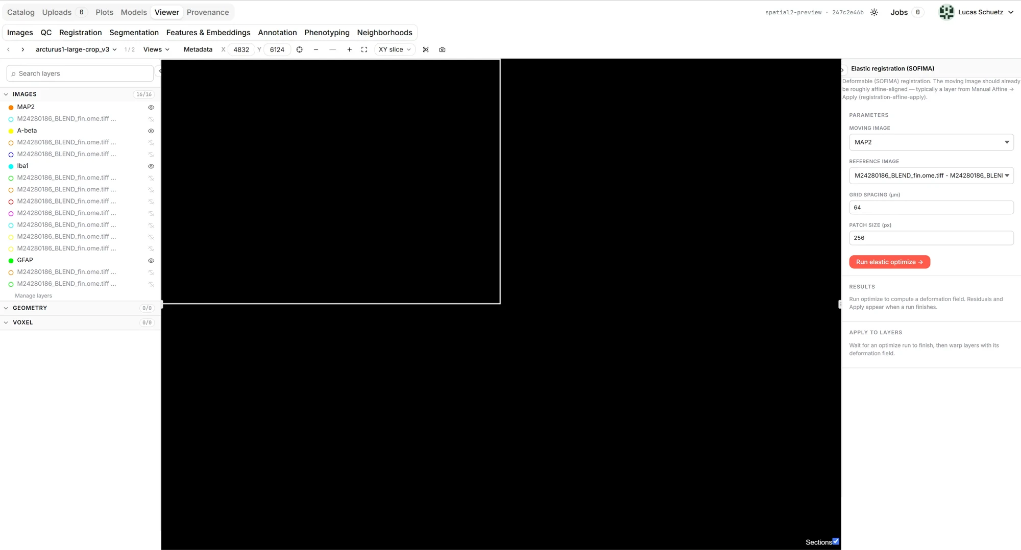
Correct complex local deformation across consecutive staining cycles, across different protocols on the same section, and across consecutive physical sections. Sectioning, hydration and shearing deform tissue locally, and a rigid or affine alignment cannot correct that. Elastic registration can, at any image size, which keeps cross-talk out of the marker table.
- Cross-cycle and cross-protocol
- Cross-section alignment
- Any image size
- Proteomics and transcriptomics in one frame
Phenotyping
Gate, cluster, compare
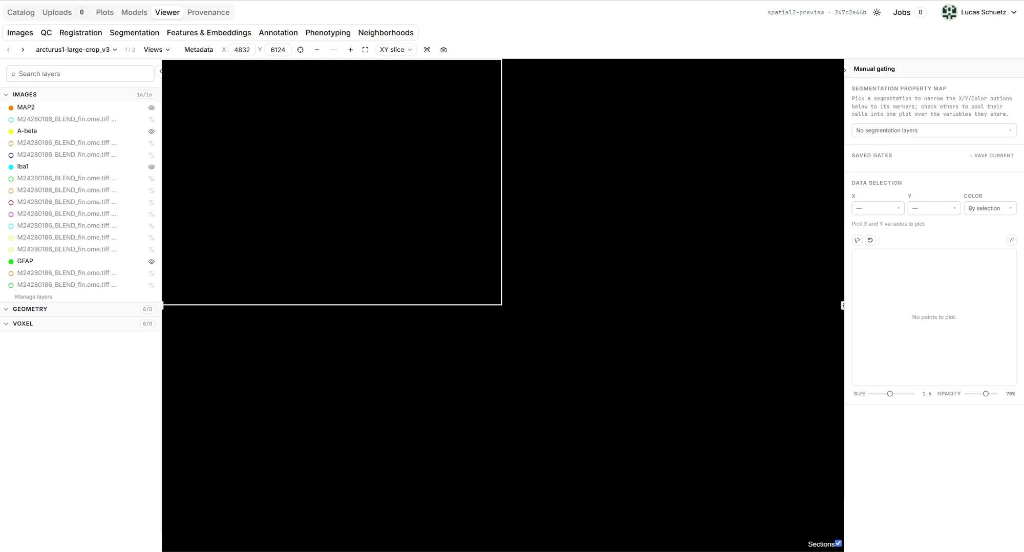
Combine manual gating, automated clustering and marker-independent tissue segmentation to group cells into phenotypes that mean something biologically. Then go past the cell table: shape, size, branching, neighbourhood composition and distance to lesion are measured per cell, so comparisons across conditions and cohorts use tissue architecture.
- Manual and hierarchical gating
- Automated clustering
- Tissue-level segmentation
- Morphometric features per cell
- Neighbourhood composition and distance to lesion
- Comparison across conditions and cohorts
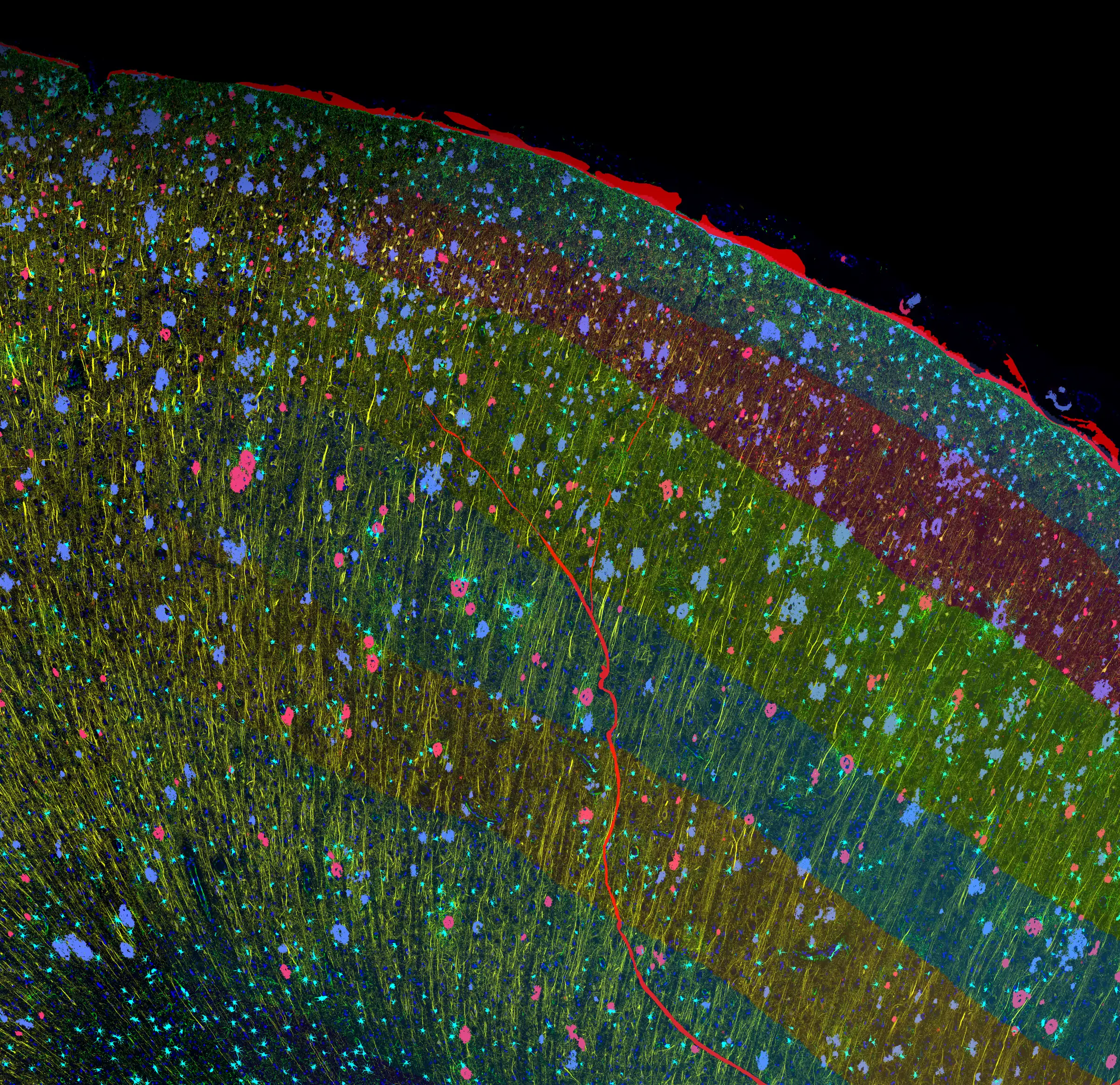
Neuropathology
Aggregates, classified and put in context
Classify pathological protein aggregates of amyloid β, phospho-tau, α-synuclein and TDP-43, and characterise the cells in their microenvironment. Dense-core versus diffuse plaques, tangles versus neuropil threads.
- Aggregate classification
- Plaque and tangle subtypes
- Microenvironment characterisation
- Region-level statistics
Custom models
When the pre-trained model is not enough
Annotate a small region of your own tissue, train a segmentation model on it, and use it alongside the pre-trained ones. Every training run keeps its loss curve, accuracy and sample count, so you always know which model produced a result.
- Train on your own stain
- A few dozen annotations to start
- Auditable training runs
- Apply to a whole cohort
Formats and instruments
Instruments
Akoya Phenocycler · Bruker Spatial Biology CosMx and CellScape · Lunaphore COMET · 10x Genomics Visium, Visium HD and Xenium · Vizgen MERSCOPE
File formats
OME-TIFF · TIFF series · Zeiss CZI · Leica LIF · dense image stacks and sparse coordinate lists. New formats are added on request.
Runs in your browser
Any modern browser
Processing happens on our GPUs, so the machine on your desk does not matter.
Any dataset size
Whole slides, cohorts and volumetric data. Nothing is limited by what fits in memory.
Explore before you commit
Try settings on a region of a slide before running the whole section.